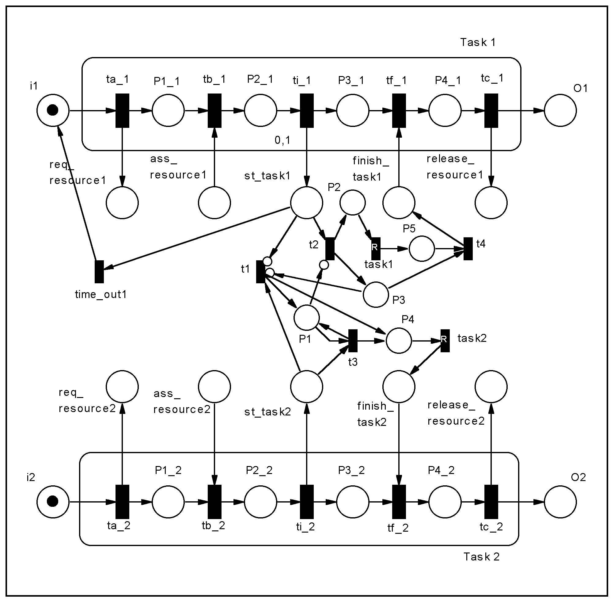
Figure 16: Coordination Machanism for Task 1 before Task 2.
Differently from the previous relation (after), the restriction
here occurs on the execution of Task 1, which cannot be performed if Task
2 has been executed. There is no restriction on the execution of Task2
(i.e., Task2 does not have to wait for the execution of Task1, as was the
case for Task2 after Task1). From the temporal logic point of view,
the difference between these two relations may not be significant, but
it generates totally different coordination mechanisms.
The modeled coordination mechanism uses inhibitor arcs. An inhibitor
arc connects a place P with a transition t and enables t
only if P has no tokens and is represented with a circle on the
edge. The core of the model is transition t1 (Figure 16),
which determines the execution of Task 2 and is inhibited if there is any
token in start_task1 or P3 (Task 1 is ready or being executed,
respectively). The firing of t1 puts a token in P1, inhibiting
the firing of t2 and, consequently, the execution of Task 1. If
Task 2 hasn't been executed yet (token in P1), t2 can be
fired, sending tokens to P2, which enables task2, and to
P3, which inhibits t1. At the end of Task 1 t4 is
fired, emoving the token from P3. Transition t3 enables other
executions of Task 2 (after the first one, that puts a token in P1),
which can happen independently of the pesence of tokens in start_task1
(Task 1 will not happen anymore). It is important to use a timeout to ensure
that Task 1 returns to its initial state when it cannot be executed anymore.
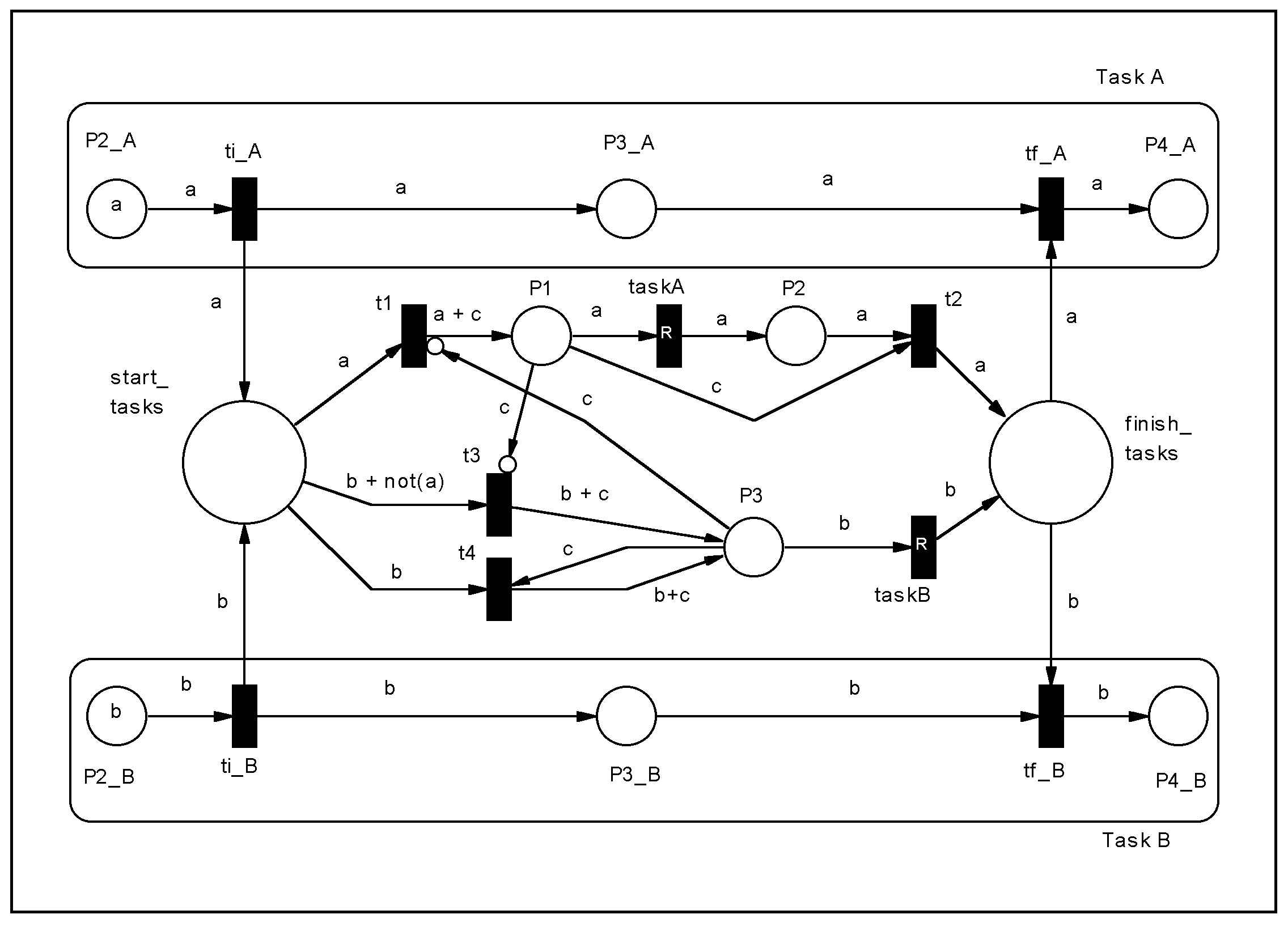
The model using high level PN is shown in Figure 17.
Besides inhibitor arcs, an arc with expression b + not(a) is used
to enable t3 only if thee is a token of color b and no one
of color a in place start_tasks.